Estimating Transfer Function Models from a Real Aero-thermal Channel
This example shows how to develop and analyze simple models from a real Aero-thermal Channel. We start with a brief description of the process, import the data and then a transfer function model is estimated and validated by using traditional model validation tests.
Contents
System Description
This demo uses the data collected from an aero-thermal channel (PT326). The process works as follows: air is fanned through a tube and heated at the inlet. The air temperature is measured by a thermocouple at the outlet. The input is the voltage over the heating device, which is just a mesh of resistor wires. The output is the outlet air temperature or rather the voltage from the thermocouple.
Loading the Data for Analysis
First load the data to the MATLAB Workspace. Two sets of data are available, the first will be used to estimate a model while the second will be reserved for model cross-validation. Note that the mean and linear trend of the signals have been previously removed from the data so that no further pre-processing of the data is required.
load contsid_dryer;
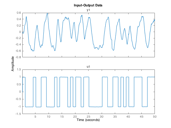
Matrix ze = [ye ue] contains 1905 output/input data measurements. The input ue was generated as a PRBS of maximum length. The sampling interval Ts is 0.1 seconds. The first step is to set up the data as an iddata object data_est which will be used to estimate a model.
data_est = iddata(ze(:,1),ze(:,2),Ts,'InterSample','zoh');
Matrix zv = [yv uv] contains the validation data set. It contains also 1905 measurements collected in the same conditions as the estimation data set ze. We also create a data object data_valid which will be used to validate the model.
data_valid = iddata(zv(:,1),zv(:,2),Ts,'InterSample','zoh');
Let us plot a snapshot of the estimation data set.
idplot(data_est,1:500)
Model Estimation
The best model structure was first determined (run contsid_tutorial6). A simple first-order model with 5 samples for the delay can be selected.
We just need then to specify the triad nn=[nb nf nk] where the first two indices define the number of parameters to be estimated for the numerator and denominator respectively of the transfer function model while nk defines the number of samples for the time-delay. The Simple Refined Instrumental Variable function SRIVC is then used to estimate a first-order transfer function model plus delay .
Msrivc = srivc(data_est,[1 1 5]);
The estimated parameters together with their standard deviation can be displayed:
present(Msrivc);
Msrivc =
Continuous-time OE model:  y(t) = [B(s)/F(s)]u(t)
  B(s) = 0.7607 (+/- 0.006844)

  F(s) = s + 1.487 (+/- 0.01637)

Input delays (listed by channel): 0.5
Parameterization:
   Polynomial orders:   nb=1   nf=1   nk=0
   Number of free coefficients: 2
   Use "polydata", "getpvec", "getcov" for parameters and their uncertainties.

Status:
Estimated using Contsid SRIVC method on time domain data.
Fit to estimation data: 77.96
FPE: 6.228e-03, MSE 6.215e-03
More information in model's "Report" property.
Model Validation
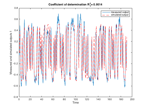
How good is this model? One way to find out is to simulate it and compare the model output with the measured output. This can be easily done by using the COMPAREC function. We first use the estimation data set that was used to build the model. It can be noticed that the agreement between the two outputs is quite good.
comparec(data_est,Msrivc);
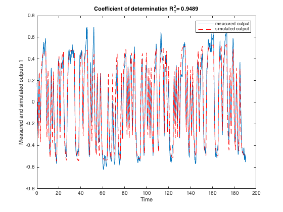
We then perform a cross-validation test. Let us compare the measured and simulated outputs. From the new figure, it can be observed that the agreement between the two outputs is also quite good.
comparec(data_valid,Msrivc);
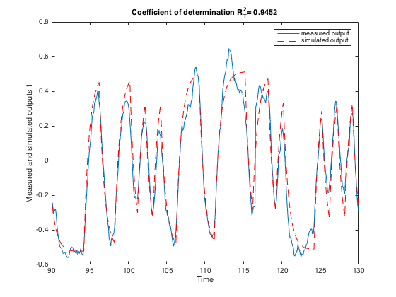
Let us compare the measured and simulated outputs on a smaller portion of the validation data. The fit is clearly quite good. The model is able to reproduce the process output on a data that has not been used to estimate the parameters.
comparec(data_valid,Msrivc,901:1300);
Additional Information
For more information on identification of continuous-time dynamic models visit the CONTSID Toolbox web page.